External libraries#

#

BB1000 Programming in Python KTH

layout: false

Learning outcomes:

numpy
pandas
matplotlib

What can you do with Python libraries#

This year’s Nobel Prize in economics was awarded to a Python convert

https://qz.com/1417145/economics-nobel-laureate-paul-romer-is-a-python-programming-convert/

Instead of using Mathematica, Romer discovered that he could use a Jupyter notebook for sharing his research. Jupyter notebooks are web applications that allow programmers and researchers to share documents that include code, charts, equations, and data. Jupyter notebooks allow for code written in dozens of programming languages. For his research, Romer used Python—the most popular language for data science and statistics.

What can you do with Python libraries#

Take a picture of a black hole

https://static.projects.iq.harvard.edu/files/styles/os_files_xlarge/public/eht/files/20190410-78m-800x466.png?m=1554877319&itok=fLnjP-iS

https://doi.org/10.3847/2041-8213/ab0e85

Software: DiFX (Deller et al. 2011), CALC, PolConvert (Martí-Vidal et al. 2016), HOPS (Whitney et al. 2004), CASA (McMullin et al. 2007), AIPS (Greisen 2003), ParselTongue (Kettenis et al. 2006), GNU Parallel (Tange 2011), GILDAS, eht-imaging (Chael et al. 2016, 2018), Numpy (van der Walt et al. 2011), Scipy (Jones et al. 2001), Pandas (McKinney 2010), Astropy (The Astropy Collaboration et al. 2013, 2018), Jupyter (Kluyver et al. 2016), Matplotlib (Hunter 2007).

What is a library?#

A file
A directory
Builtin
Standard library (requires import)
External libraries (requires install)

Builtins#

>>> dir(__builtins__) 
[
...
 'abs', 'all', 'a
ny', 'ascii', 'bin', 'bool', 'bytearray', 'bytes', 'callable', 'chr', 'classmetho
d', 'compile', 'complex', 'copyright', 'credits', 'delattr', 'dict', 'dir', 'divm
od', 'enumerate', 'eval', 'exec', 'exit', 'filter', 'float', 'format', 'frozenset
', 'getattr', 'globals', 'hasattr', 'hash', 'help', 'hex', 'id', 'input', 'int', 
'isinstance', 'issubclass', 'iter', 'len', 'license', 'list', 'locals', 'map', 'm
ax', 'memoryview', 'min', 'next', 'object', 'oct', 'open', 'ord', 'pow', 'print',
 'property', 'quit', 'range', 'repr', 'reversed', 'round', 'set', 'setattr', 'sli
ce', 'sorted', 'staticmethod', 'str', 'sum', 'super', 'tuple', 'type', 'vars', 'z
ip']                            

Standard library#

Included in all distributions, but requires an import statement for access

>>> import math
>>> math.pi
3.141592653589793

https://docs.python.org/3/library/

---

External Python libraries#

NumPy: ‘Numerical python’, linear algebra, https://www.numpy.org/
Pandas: High-level library for tabular data, https://pandas.pydata.org/
Matplotlib: fundamental plotting module, https://matplotlib.org/

Are you a math genius?#

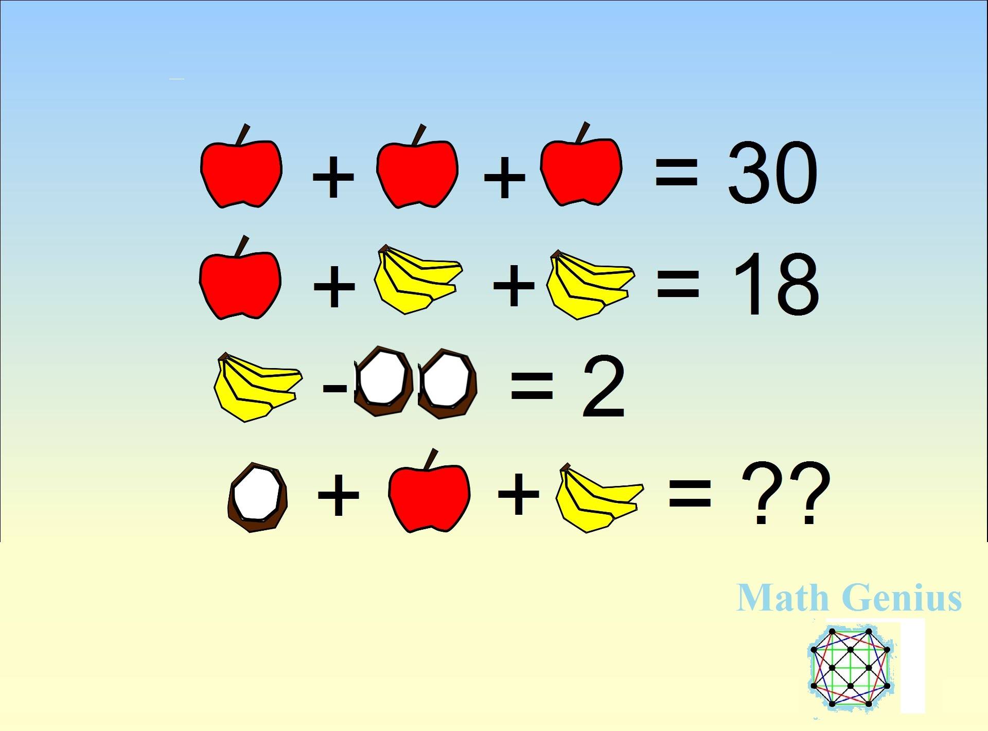
First three rows a linear system of equations
Identify the coefficient matrix and right-hand side
Last line represents an expression of the solutions

(1)#\[\begin{pmatrix} 3 &0 &0 \\\ 1 &8 &0 \\\ 0 &4 &-2 \end{pmatrix}\]

(2)#\[\begin{pmatrix} a\\\ b \\\ c \end{pmatrix}\]

(3)#\[\begin{pmatrix} 30\\\ 18 \\\ 2 \end{pmatrix}\]

$$ $$ a + 3b + c = ? $$

Linear Algebra in Python: NumPy#

Libraries provided by numpy provide computational speeds close to compiled languages
Generally written in C
From a user perspective they are imported as any python module
http://www.numpy.org

Creating arrays#

one- and two-dimensional

>>> import numpy
>>> a = numpy.zeros(3)
>>> a  
array([0., 0., 0.])
>>> b = numpy.zeros((3, 3))
>>> b  
array([[0., 0., 0.],
       [0., 0., 0.],
       [0., 0., 0.]])

Copying arrays#

>>> x = numpy.zeros(2)
>>> y = x
>>> x[0] = 1
>>> x
array([1., 0.])
>>> y
array([1., 0.])

Note that assignment (like lists) here is by reference

>>> x is y
True

Numpy array copy method

>>> y = x.copy()
>>> x is y
False

Filling arrays#

linspace returns an array with sequence data

>>> numpy.linspace(0,1,6) 
array([0. , 0.2, 0.4, 0.6, 0.8, 1. ])

arange is a similar function

>>> numpy.arange(0, 1, 0.2) 
array([0. , 0.2, 0.4, 0.6, 0.8])

Arrays from list objects#

>>> la=[1., 2., 3.]
>>> a=numpy.array(la)
>>> a
array([1., 2., 3.])

>>> lb=[4., 5., 6.]
>>> ab=numpy.array([la,lb])
>>> ab
array([[1., 2., 3.],
       [4., 5., 6.]])

Arrays from file data:#

Using numpy.loadtxt

#a.dat
1 2 3
4 5 6

>>> a = numpy.loadtxt('a.dat')
>>> a
array([[1., 2., 3.],
       [4., 5., 6.]])

If you have a text file with only numerical data arranged as a matrix: all rows have the same number of elements

Reshaping#

by changing the shape attribute

>>> ab.shape
(2, 3)
>>> ab = ab.reshape((6,))
>>> ab.shape
(6,)

with the reshape method

>>> ba = ab.reshape((3, 2))
>>> ba
array([[1., 2.],
       [3., 4.],
       [5., 6.]])

Views of same data#

ab and ba are different objects but represent different views of the same data

>>> ab[0] = 0
>>> ab
array([0., 2., 3., 4., 5., 6.])
>>> ba
array([[0., 2.],
       [3., 4.],
       [5., 6.]])

Array indexing and slicing#

like lists

a[2: 4] is an array slice with elements a[2] and a[3]
a[n: m] has size m-n
a[-1] is the last element of a
a[:] are all elements of a

Matrix operations#

From mathematics:

\[C_{ij} = \sum_k A_{ik}B_{kj}\]

explicit looping (slow):

import time

import numpy

n = 256
a = numpy.ones((n, n))
b = numpy.ones((n, n))
c = numpy.zeros((n, n))
t1 = time.time()
for i in range(n):
    for j in range(n):
        for k in range(n):
            c[i, j] += a[i, k]*b[k, j]
t2 = time.time()
print("Loop timing", t2-t1)

using numpy

import time

import numpy

n = 256
a = numpy.ones((n, n))
b = numpy.ones((n, n))
t1 = time.clock()
c = a @ b
t2 = time.clock()
print("dot timing", t2-t1)

@ is a matrix multiplication operator, same as

c = numpy.dot(a, b)

More vector operations#

Scalar multiplication a * 2
Scalar addition a + 2
Power (elementwise) a**2

Note that for objects of ndarray type, multiplication means elementwise multplication and not matrix multiplication

Vectorized elementary functions#

>>> v = numpy.arange(0, 1, .2)
>>> v
array([0. , 0.2, 0.4, 0.6, 0.8])

–

>>> numpy.cos(v)
array([1.        , 0.98006658, 0.92106099, 0.82533561, 0.69670671])

–

>>> numpy.sqrt(v)
array([0.        , 0.4472136 , 0.63245553, 0.77459667, 0.89442719])

–

>>> numpy.log(v) 
...
array([       -inf, -1.60943791, -0.91629073, -0.51082562, -0.22314355])

More linear algebra#

Solve a linear system of equations $$Ax = b$$

–

    x = numpy.linalg.solve(A, b)

–

Determinant of a matrix

$$det(A)$$

–

    x = numpy.linalg.det(A)

Inverse of a matrix $$A^{-1}$$

–

    x = numpy.linalg.inverse(A)

–

Eigenvalues of a matrix

$$Ax = x\lambda$$

–

    x, l = numpy.linalg.eig(A)

References#

http://www.numpy.org
http://www.scipy-lectures.org/intro/numpy/index.html
Videos: https://pyvideo.org/search.html?q=numpy

Matplotlib#

The standard 2D-plotting library in Python
Production-quality graphs
Interactive and non-interactive use
Many output formats
Flexible and customizable

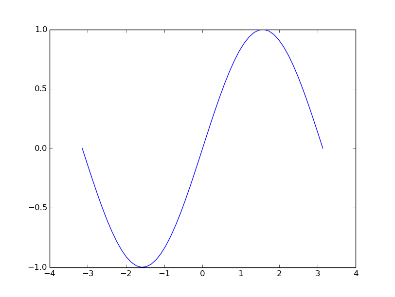
First example#

The absolute minimum you need to know#

You have a set of points (x,y) on file data.txt

-3.141593 -0.000000
-3.013364 -0.127877
-2.885136 -0.253655
...
3.141593 0.000000

–

How do you get to this

Next#

Import the plotting library

>>> import matplotlib.pyplot as plt
>>> import numpy as np

–

Load the data from file

>>> data = np.loadtxt('data.txt') 

–

Call the plot function

>>> plt.plot(data[:, 0], data[:, 1]) 

–

Show the result

>>> plt.show() 

Next?#

In practice#

How do you do when need a particlar type of figure?

Go to the matplotlib gallery: http://matplotlib.org/gallery
Try some exercises at http://scipy-lectures.github.io/intro/matplotlib/matplotlib.html#other-types-of-plots-examples-and-exercises
See also: https://realpython.com/python-matplotlib-guide/

The `pandas` module#

Setup:

>>> import pandas as pd
>>> import numpy as np
>>> import matplotlib.pyplot as plt

Two main data structures

Series
Data frames

Series#

One-dimensional labeled data

>>> s = pd.Series([0.1, 0.2, 0.3, 0.4])
>>> print(s)
0    0.1
1    0.2
2    0.3
3    0.4
dtype: float64

–

>>> s.index
RangeIndex(start=0, stop=4, step=1)

–

>>> s.values
array([0.1, 0.2, 0.3, 0.4])

indices can be labels (like a dict with order)

>>> s = pd.Series(np.arange(4), index=['a', 'b', 'c', 'd'])
>>> print(s)
a    0
b    1
c    2
d    3
dtype: int64
>>> print(s['d'])
3
>>>

–

Initialize with dict

>>> s = pd.Series({'a': 1, 'b': 2, 'c': 3, 'd': 4})
>>> print(s)
a    1
b    2
c    3
d    4
dtype: int64

–

Indexing as a dict

>>> print(s['a'])
1

Elementwise operations

>>> s * 100
a    100
b    200
c    300
d    400
dtype: int64
>>>

–

Slicing

>>> s['b': 'c']
b    2
c    3
dtype: int64
>>>

List indexing

>>> print(s[['b', 'c']])
b    2
c    3
dtype: int64
>>>

–

Bool indexing

>>> print(s[s>2])
c    3
d    4
dtype: int64
>>>

–

Other operations

>>> s.mean()
2.5
>>>

Alignment on indices

>>> s['a':'b'] + s['b':'c']  
a   NaN
b   4.0
c   NaN
dtype: float64

DataFrames#

Tabular data structure (like spreadsheet, sql table)
Multiple series with common index

>>> data = {'country': ['Belgium', 'France', 'Germany', 'Netherlands', 'United Kingdom'],
...        'population': [11.3, 64.3, 81.3, 16.9, 64.9],
...        'area': [30510, 671308, 357050, 41526, 244820],
...        'capital': ['Brussels', 'Paris', 'Berlin', 'Amsterdam', 'London']}
>>>

–

>>> countries = pd.DataFrame(data)
>>> countries
          country  population    area    capital
0         Belgium        11.3   30510   Brussels
1          France        64.3  671308      Paris
2         Germany        81.3  357050     Berlin
3     Netherlands        16.9   41526  Amsterdam
4  United Kingdom        64.9  244820     London

Attributes: index, columns, dtypes, values

>>> countries.index
RangeIndex(start=0, stop=5, step=1)

–

>>> countries.columns
Index(['country', 'population', 'area', 'capital'], dtype='object')

–

>>> countries.dtypes
country        object
population    float64
area            int64
capital        object
dtype: object
>>>

–

>>> countries.values
array([['Belgium', 11.3, 30510, 'Brussels'],
       ['France', 64.3, 671308, 'Paris'],
       ['Germany', 81.3, 357050, 'Berlin'],
       ['Netherlands', 16.9, 41526, 'Amsterdam'],
       ['United Kingdom', 64.9, 244820, 'London']], dtype=object)

Info

>>> countries.info()
<class 'pandas.core.frame.DataFrame'>
RangeIndex: 5 entries, 0 to 4
Data columns (total 4 columns):
 #   Column      Non-Null Count  Dtype  
---  ------      --------------  -----  
 0   country     5 non-null      object 
 1   population  5 non-null      float64
 2   area        5 non-null      int64  
 3   capital     5 non-null      object 
dtypes: float64(1), int64(1), object(2)
memory usage: 288.0+ bytes

RangeInde: 5 entries, 0 to 4
Data columns (total 4 columns):
area          5 non-null int64
capital       5 non-null object
country       5 non-null object
population    5 non-null float64
dtypes: float64(1), int64(1), object(2)
memory usage: 200.0 bytes
>>>

Set a column as index

>>> countries
          country  population    area    capital
       Belgium        11.3   30510   Brussels
        France        64.3  671308      Paris
       Germany        81.3  357050     Berlin
   Netherlands        16.9   41526  Amsterdam
United Kingdom        64.9  244820     London

–

>>> countries = countries.set_index('country')

–

>>> countries
                population    area    capital
country                                      
Belgium               11.3   30510   Brussels
France                64.3  671308      Paris
Germany               81.3  357050     Berlin
Netherlands           16.9   41526  Amsterdam
United Kingdom        64.9  244820     London

Access a single series in a table

>>> print(countries['area'])
country
Belgium            30510
France            671308
Germany           357050
Netherlands        41526
United Kingdom    244820
Name: area, dtype: int64

–

>>> print(countries['capital']['France'])
Paris

–

Arithmetic expressions (population density)

>>> print(countries['population']/countries['area']*10**6)
country
Belgium           370.370370
France             95.783158
Germany           227.699202
Netherlands       406.973944
United Kingdom    265.092721
dtype: float64
>>>

Add new column

>>> countries['density'] =  countries['population']/countries['area']*10**6
>>> countries 
                    population    area    capital     density
    country
    Belgium               11.3   30510   Brussels  370.370370
    France                64.3  671308      Paris   95.783158
    Germany               81.3  357050     Berlin  227.699202
    Netherlands           16.9   41526  Amsterdam  406.973944
    United Kingdom        64.9  244820     London  265.092721

–

Filter data

>>> countries[countries['density'] > 300] 
                 population   area    capital     density
    country
    Belgium            11.3  30510   Brussels  370.370370
    Netherlands        16.9  41526  Amsterdam  406.973944

Sort data

>>> countries.sort_values('density', ascending=False) 
                    population    area    capital     density
    country
    Netherlands           16.9   41526  Amsterdam  406.973944
    Belgium               11.3   30510   Brussels  370.370370
    United Kingdom        64.9  244820     London  265.092721
    Germany               81.3  357050     Berlin  227.699202
    France                64.3  671308      Paris   95.783158

–

Statistics

>>> countries.describe() 
           population           area     density
    count    5.000000       5.000000    5.000000
    mean    47.740000  269042.800000  273.183879
    std     31.519645  264012.827994  123.440607
    min     11.300000   30510.000000   95.783158
    25%     16.900000   41526.000000  227.699202
    50%     64.300000  244820.000000  265.092721
    75%     64.900000  357050.000000  370.370370
    max     81.300000  671308.000000  406.973944

Plotting

>>> countries.plot()  

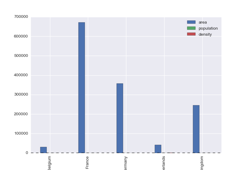
Plotting barchart

>>> countries.plot(kind='bar')  

Features#

like numpy arrays with labels
supported import/export formats: CSV, SQL, Excel…
support for missing data
support for heterogeneous data
merging data
reshaping data
easy plotting

BB1000 lecture notes

External libraries

Contents

External libraries#

#

What can you do with Python libraries#

What can you do with Python libraries#

What is a library?#

Builtins#

Standard library#

External Python libraries#

Are you a math genius?#

Linear Algebra in Python: NumPy#

Creating arrays#

Copying arrays#

Filling arrays#

Arrays from list objects#

Arrays from file data:#

Reshaping#

Views of same data#

Array indexing and slicing#

Matrix operations#

More vector operations#

Vectorized elementary functions#

More linear algebra#

References#

Matplotlib#

First example#

The absolute minimum you need to know#

Next#

Next?#

Refinement#

In practice#

The `pandas` module#

Series#

DataFrames#

Features#

BB1000 lecture notes

External libraries

Contents

External libraries#

#

What can you do with Python libraries#

What can you do with Python libraries#

What is a library?#

Builtins#

Standard library#

External Python libraries#

Are you a math genius?#

Linear Algebra in Python: NumPy#

Creating arrays#

Copying arrays#

Filling arrays#

Arrays from list objects#

Arrays from file data:#

Reshaping#

Views of same data#

Array indexing and slicing#

Matrix operations#

More vector operations#

Vectorized elementary functions#

More linear algebra#

References#

Matplotlib#

First example#

The absolute minimum you need to know#

Next#

Next?#

Refinement#

In practice#

The pandas module#

Series#

DataFrames#

Features#

The `pandas` module#